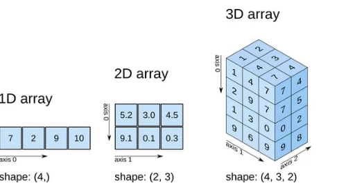
텐서(Tensor)
텐서(tensor)는 배열(array)이나 행렬(matrix)과 매우 유사한 특수한 자료구조이다.
PyTorch에서는 텐서를 사용하여 모델의 입력(input)과 출력(output), 그리고 모델의 매개변수들을 부호화(encode)한다.
텐서는 GPU나 다른 하드웨어 가속기에서 실행할 수 있다는 점만 제외하면 NumPy의 ndarray와 유사한데, 텐서는 또한 뒤에서 살펴볼 자동 미분(automatic differentiation)에 최적화되어 있으므로, ndarray에 익숙하다면 Tensor API를 바로 사용할 수 있을 것이다.
| import torch import numpy as np |
텐서(tensor) 초기화
이번 섹션에서는 다양한 방법을 이용하여 tensor를 초기화를 진행해보려고 한다.
List 배열로부터 생성하기
텐서는 List로 생성할 수 있다. (그 반대도 가능함)
| data = [[1, 2],[3, 4]] x_data = torch.tensor(data) print(x_data) # list로부터 tensor 생성 print(x_data.tolist()) # tensor에서 list로 다시 전환 |
tensor([[1, 2],
        [3, 4]])
[[1, 2], [3, 4]]
NumPy 배열로부터 생성하기
텐서는 NumPy 배열로 생성할 수 있다 . ( 그 반대도 가능함 )
| data = [[1, 2],[3, 4]] np_array = np.array(data) x_np = torch.from_numpy(np_array) print(x_np) print(x_np.numpy()) |
tensor([[1, 2],
        [3, 4]])
[[1 2]
 [3 4]]
무작위(random) 또는 상수(constant) 값을 사용하기:
shape 은 텐서의 차원(dimension)을 나타내는 튜플(tuple)로, 아래 함수들에서는 출력 텐서의 차원을 결정한다.
| shape = (2,3) rand_tensor = torch.rand(shape) ones_tensor = torch.ones(shape) zeros_tensor = torch.zeros(shape) print(f"Random Tensor: \n {rand_tensor} \n") print(f"Ones Tensor: \n {ones_tensor} \n") print(f"Zeros Tensor: \n {zeros_tensor}") |
Random Tensor:
 tensor([[0.7462, 0.6793, 0.0487],
        [0.3189, 0.6058, 0.1788]])

Ones Tensor:
 tensor([[1., 1., 1.],
        [1., 1., 1.]])

Zeros Tensor:
 tensor([[0., 0., 0.],
        [0., 0., 0.]])
| a = torch.ones_like(rand_tensor) print(a) |
tensor([[1., 1., 1.],
        [1., 1., 1.]])
텐서의 속성(Attribute)
텐서의 속성은 텐서의 모양(shape), 자료형(datatype) 및 어느 장치(device)에 저장되는지를 나타낸다.
| tensor = torch.rand(3,4) print(f"Shape of tensor: {tensor.shape}") print(f"Datatype of tensor: {tensor.dtype}") print(f"Device tensor is stored on: {tensor.device}") |
Shape of tensor: torch.Size([3, 4])
Datatype of tensor: torch.float32
Device tensor is stored on: cpu
텐서 연산
NumPy식의 표준 인덱싱과 슬라이싱:
| tensor = torch.ones(4, 4) print(tensor) print('First row: ',tensor[0]) print('First column: ', tensor[:, 0]) print('Last column:', tensor[:, -1]) tensor[:,1] = 0 print(tensor) |
tensor([[1., 1., 1., 1.],
        [1., 1., 1., 1.],
        [1., 1., 1., 1.],
        [1., 1., 1., 1.]])
First row:  tensor([1., 1., 1., 1.])
First column:  tensor([1., 1., 1., 1.])
Last column: tensor([1., 1., 1., 1.])
tensor([[1., 0., 1., 1.],
        [1., 0., 1., 1.],
        [1., 0., 1., 1.],
        [1., 0., 1., 1.]])
텐서 합치기
torch.cat 을 사용하여 주어진 차원에 따라 일련의 텐서를 연결할 수 있다.
| t1 = torch.cat([tensor, tensor, tensor], dim=1) print(t1) |
tensor([[1., 0., 1., 1., 1., 0., 1., 1., 1., 0., 1., 1.],
        [1., 0., 1., 1., 1., 0., 1., 1., 1., 0., 1., 1.],
        [1., 0., 1., 1., 1., 0., 1., 1., 1., 0., 1., 1.],
[1., 0., 1., 1., 1., 0., 1., 1., 1., 0., 1., 1.]])| t1 = torch.cat([tensor, tensor, tensor], dim=0) print(t1) |
tensor([[1., 0., 1., 1.],
        [1., 0., 1., 1.],
        [1., 0., 1., 1.],
        [1., 0., 1., 1.],
        [1., 0., 1., 1.],
        [1., 0., 1., 1.],
        [1., 0., 1., 1.],
        [1., 0., 1., 1.],
        [1., 0., 1., 1.],
        [1., 0., 1., 1.],
        [1., 0., 1., 1.],
        [1., 0., 1., 1.]])
산술 연산(Arithmetic operations)
| import torch a = torch.tensor([1,2,3]) b = torch.tensor([3,4,5]) # 두 텐서간의 합 print("a + b : ", a+b) # 두 텐서간의 차 print("a - b : ", a-b) |
a + b :  tensor([4, 6, 8])
a - b : tensor([-2, -2, -2])| # 두 텐서 간의 행렬 곱(matrix multiplication)을 계산합니다. y1, y2, y3은 모두 같은 값을 갖습니다. data = torch.tensor([[1,2],[3,4]]) print("data : ", data) print("data.T : ", data.T) y1 = data @ data.T y2 = data.matmul(data.T) y3 = torch.matmul(data, data.T) print(y1) print(y2) print(y3) # 요소별 곱(element-wise product)을 계산합니다. z1, z2, z3는 모두 같은 값을 갖습니다. z1 = data * data z2 = data.mul(data) z3 = torch.mul(data, data) print(z1) print(z2) print(z3) |
data :  tensor([[1, 2],
        [3, 4]])
data.T :  tensor([[1, 3],
        [2, 4]])
tensor([[ 5, 11],
        [11, 25]])
tensor([[ 5, 11],
        [11, 25]])
tensor([[ 5, 11],
        [11, 25]])
tensor([[ 1,  4],
        [ 9, 16]])
tensor([[ 1,  4],
        [ 9, 16]])
tensor([[ 1,  4],
        [ 9, 16]])
비선형 연산
| input = torch.tensor([-2, -1, 0, 1, 2, 3]).float() #ReLU import torch ReLU = torch.nn.ReLU() print("ReLU : ", ReLU(input)) #softmax m = torch.nn.Softmax(dim=0) input = torch.tensor([-2, -1, 1, 2, 3]).float() print("softamx : " , m(input)) #sigmoid print("sigmoid : " , torch.sigmoid(input)) |
ReLU :  tensor([0., 0., 0., 1., 2., 3.])
softamx :  tensor([0.0044, 0.0120, 0.0886, 0.2407, 0.6543])
sigmoid :  tensor([0.1192, 0.2689, 0.7311, 0.8808, 0.9526])
단일-요소(single-element) 텐서
텐서의 모든 값을 하나로 집계(aggregate)하여 요소가 하나인 텐서의 경우, item() 을 사용하여 Python 숫자 값으로 변환할 수 있다.
| data |
tensor([[1, 2],
        [3, 4]])
| agg = data.sum() print(agg, type(agg)) agg_item = agg.item() print(agg_item, type(agg_item)) |
tensor(10) <class 'torch.Tensor'>
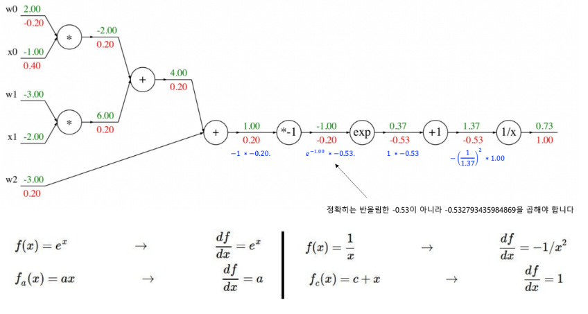
10 <class 'int'>역전파(Backpropagation)
tensor를 사용하면 이전에 배웠던 역전파를 굉장히 간단하게 사용할 수 있다.
| a = torch.tensor([1.0,2.0,3.0], requires_grad=True) b = torch.tensor([2.0,3.0,4.0], requires_grad=True) c = torch.tensor([4.0,5.0,6.0], requires_grad=True) d = torch.tensor([7.0,8.0,9.0], requires_grad=True) print(a.grad) |
None
덧셈에 대한 Auto Grad
| y = a+b print("y : ", y.data) print("y_grad_fn : ", y.grad_fn) |
y :  tensor([3., 5., 7.])
y_grad_fn :  <AddBackward0 object at 0x7de33ad91b10>
뺄셈에 대한 Auto Grad
| y = y-c print("y : ", y.data) print("y_grad_fn : ", y.grad_fn) |
y :  tensor([-1.,  0.,  1.])
y_grad_fn :  <SubBackward0 object at 0x7de40bedcd60>
곱셈에 대한 Auto Grad
| y = y*d print("y : ", y.data) print("y_grad_fn : ", y.grad_fn) |
y :  tensor([-7.,  0.,  9.])
y_grad_fn :  <MulBackward0 object at 0x7de33ad92c50>
RELU 연산에 대한 Auto Grad
| y = ReLU(y) print("y : ", y.data) print("y_grad_fn : ", y.grad_fn) |
y :  tensor([0., 0., 9.])
y_grad_fn :  <ReluBackward0 object at 0x7de33ad93ee0>
Summation에 대한 Auto Grad
| y = torch.sum(y) print("y : ", y.data) print("y_grad_fn : ", y.grad_fn) |
y :  tensor(9.)
y_grad_fn :  <SumBackward0 object at 0x7de418cf4490>
Gradient 자동 계산
Gradient를 자동 계산하기 위해서는 requires_grad가 필요하다.
해당 작업을 해주지 않을 경우 오류가 발생한다.
| a = torch.tensor([1.0,2.0,3.0], requires_grad=True) b = torch.tensor([1.0,2.5,4.0], requires_grad=True) y = a*b z = y.sum() z.backward() print(a.grad) print(b.grad) |
그러나 단순히 backward() 함수를 호출하는 것만으로는 텐서 값이 자동으로 업데이트되지 않는다. backward()는 기울기를 계산하는 역할을 하지만, 실제 파라미터의 값을 변경하려면 추가적인 과정이 필요하다.
파라미터의 값을 자동으로 업데이트하려면 torch.nn.Parameter를 사용하여 텐서를 학습 가능한 파라미터로 설정해야 하며, 그 후에 옵티마이저(optimizer)를 사용하여 역전파(back-propagation) 과정을 통해 값을 조정할 수 있다. 이를 통해 기울기가 계산되고, 그 기울기를 바탕으로 파라미터의 값이 갱신된다.
optimizer는 손실 함수(loss function)를 최소화하는 방향으로 파라미터를 업데이트하여, 결과적으로 모델이 global minima(전역 최소점)에 도달할 수 있도록 돕는 역할을 한다. 여러 가지 최적화 알고리즘이 있으며, 가장 대표적인 것으로는 SGD, Adam 등이 있다. 이러한 옵티마이저는 파라미터 업데이트 규칙을 정의하며, 학습 과정을 통해 모델 성능을 점진적으로 향상시킨다.
| import torch.optim as optim device = "cuda" if torch.cuda.is_available() else "cpu" print(d) print("=" * 100) a = torch.nn.Parameter(a) b = torch.nn.Parameter(b) c = torch.nn.Parameter(c) d = torch.nn.Parameter(d) optimizer = optim.SGD([a,b,c,d], lr = 3.0) gt = torch.tensor([10.0,30.0,50.0]) y = a+b y = y-c y = y*d y = torch.sigmoid(y) loss = torch.sum(y-gt) print("loss: ", loss) loss.backward() print("a.grad: ", a.grad) print("b.grad: ", b.grad) print("c.grad: ", c.grad) print("d.grad: ", d.grad) optimizer.step() print(d) |
tensor([7., 8., 9.], requires_grad=True)
====================================================================================================
loss:  tensor(-88.4992, grad_fn=<SumBackward0>)
a.grad:  tensor([6.3715e-03, 2.0000e+00, 1.1103e-03])
b.grad:  tensor([6.3715e-03, 2.0000e+00, 1.1103e-03])
c.grad:  tensor([-6.3715e-03, -2.0000e+00, -1.1103e-03])
d.grad:  tensor([-0.0009,  0.0000,  0.0001])
Parameter containing:
tensor([7.0027, 8.0000, 8.9996], requires_grad=True)'AI' 카테고리의 다른 글
| 랭체인을 이용한 RAG (0) | 2025.04.01 |
|---|---|
| Deep Learning GPU and CPU (0) | 2025.03.28 |
| Deep Learning 개론 (0) | 2025.03.28 |
| Agents Are Not Enough, Integration of Agentic AI with 6G Networks for Mission-CriticalApplications: Use-case and Challenges 논문 리뷰 (1) | 2025.03.12 |
| AI Agent 와 AAI(Agentic AI) (0) | 2025.03.12 |


